5.11 Regression Discontinuity Design (RDD)

The Regression Discontinuity Design (RDD) is a statistical method used to estimate causal effect in situations where a treatment or intervention is assigned based on a specific threshold or cutoff point in a continuous variable.

The model can be seen as a special variant of regression analysis, where one has a clearly defined hypothesis/assumption that a given event occurs if one crosses a threshold value for a specified cutoff variable (also called the "running variable"), causing the dependent variable to make a jump either up (positive estimate) or down (negative estimate). The cutoff variable should ideally be continuous, but variables with rankable numeric values can also be used.

In practice, two separate regression curves are estimated, one for the population with a value of the cutoff variable lower than the cutoff point, and another for the group with a value higher than the cutoff limit. The estimates reported in the main table after running the command correspond to the vertical distance between the two regression curves measured at the cutoff point.

Illustration of case suitable for RDD analysis:

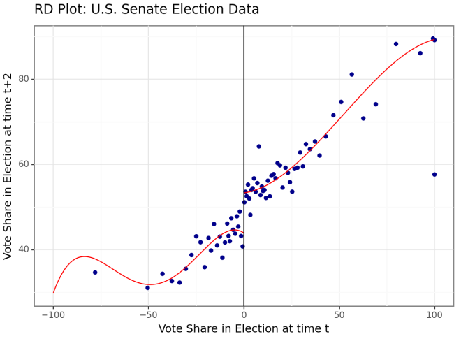This analysis looks at the effect of winning an election (margin > 0) on the election result two years later. A clear vertical jump can be seen in the plots when a positive margin is achieved, i.e., the zero point is passed (i.e., the election is won). Source: Calonico, Cattaneo & Titiunik. https://rdpackages.github.io/rdrobust/

The regression command rdd runs a so-called "Sharp Robust RDD" by default, i.e., there is a deterministic relationship. If instead, there is an assumption that there is a given probability that treatment/intervention occurs after the cutoff point (probability less than 100%), one can run a "Fuzzy Robust RDD" through the fuzzy() option. This requires the creation of a so-called treatment dummy that takes the value 1 if treatment/intervention and 0 otherwise. This dummy is specified as an argument inside the fuzzy() option.

Common to both "Sharp" and "Fuzzy" variants is that at least two variables must be specified in the rdd statement: The first variable (dependent variable) can be of any numeric format, while variable no. 2 (cutoff variable / running variable) must be either continuous or rankable. Other explanatory variables are specified as variable no. 3 and onwards. The cutoff point is set to the value 0 by default, given by variable no. 2. This can be adjusted through the cutoff() option. Otherwise, there are also the options polynomial(), derivate(), level() and cluster() that can be used to make certain adjustments in the estimation. For info about these, use the help rdd command in the analysis environment.

The hexbin command is a useful tool for seeing whether a vertical displacement of the observations for your population can be observed, which gives an indication of whether your RDD model is well suited to test your hypotheses. Hexbin is then run with the dependent variable and cutoff variable as arguments, and an anonymized scatter plot is obtained where one can observe if something systematic happens before/after the cutoff point.

Example 1: Sharp RDD

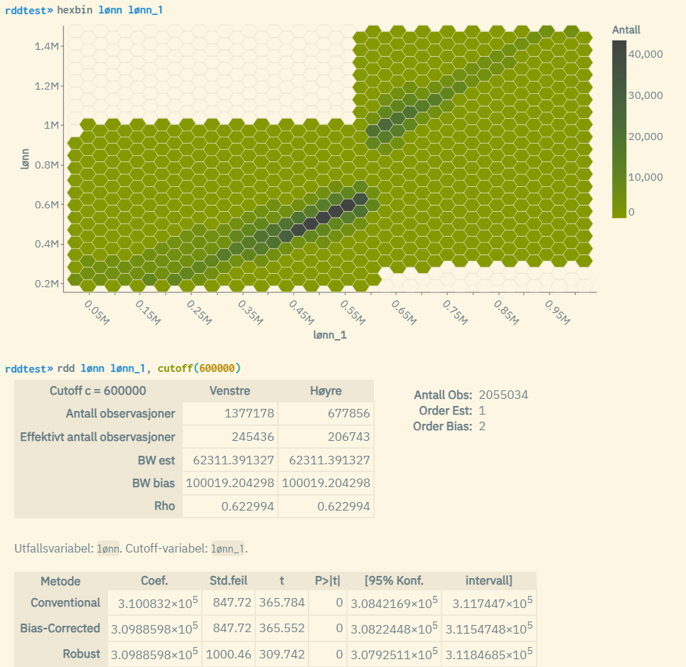The hexbin graph shows a case where there is a 100% deterministic relationship. A clear jump upward in the plots (dark color indicates strong intensity in plot occurrences) can be seen at the cutoff value 600,000. The variables "lønn" and "lønn_1" are annual salary income for a specific year and the year before, where "lønn" has been manipulated by multiplying by a factor of 1.5 if lønn_1 >= 600000. In the estimates at the bottom, one can see from the "Conventional" line that the effect of reaching an income of 600,000 the year before amounts to approximately 310000. And with a p-value equal to 0, the result is very significant.

In the example above, the cutoff limit value 600000 is used because we know that it is at this point that a shift of the regression lines can be observed. If desired, one can standardize the values of the cutoff variable "lønn_1" by subtracting 600,000 from all values. Then the cutoff limit value will be 0 instead, and the cutoff() option is not needed since 0 is the default choice for rdd. The results of the rdd run will be identical.

Example 2: Fuzzy RDD

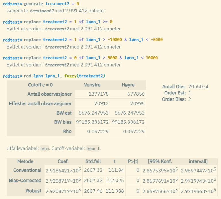Here, the cutoff variable is standardized so that the cutoff value = 0. In addition, a "treatment" variable is created that takes the values 0 or 1 both before and after the cutoff point. Then there is a non-deterministic relationship where a fuzzy model is more appropriate to use. Here too, the p-values are equal to 0, which is an indication of a good model fit.

Example 3: Sharp RDD with extra explanatory variables

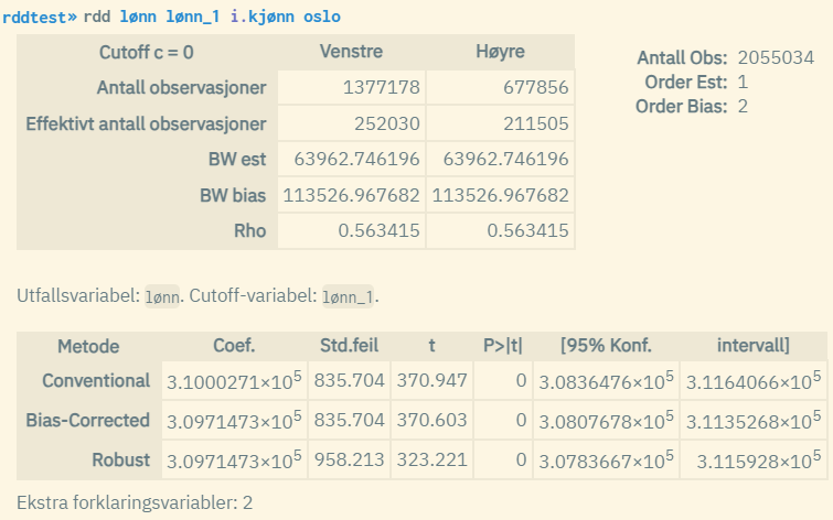In this case, the explanatory variables "kjønn" (factor variable for gender) and "oslo" (dummy for Oslo residency) are also used. This doesn't affect the estimates for the vertical displacement much. Note that estimates for the extra explanatory variables are not shown in the result. This is the standard way to report such estimates.

About the results:

Conventional: Regular RD estimate (estimate for vertical displacement at the cutoff point)
Bias-Corrected: Bias-adjusted RD estimate with regular standard errors
Robust: Bias-adjusted RD estimate with robust standard errors

Effektivt antall observasjoner: The number of observations used to estimate respectively to the left and right of the cutoff point (only the closest observations are used in the estimation)
BW est: This indicates the limit values for which observations are used in the estimation of the regular RD estimate, i.e., cutoff value +/- given value
BW bias: Indicates the limit values associated with the estimation of the bias-adjusted estimator, i.e., cutoff value +/- given value
Rho: "BW est" divided by "BW bias"
Order Est: Order of the local polynomial used to estimate the point estimator (at the cutoff point). The default value is 1, but this can be changed through the polynomial() option. The value 1 indicates local linear regression.
Order Bias: Order of the local polynomial used to estimate the bias adjustment (at the cutoff point). The default value is 2, which indicates local quadratic regression. The value is adjusted automatically according to the value of "Order Est".

$\rhd$ Practical examples: Script for reproducing the examples above

Source: The algorithms for the rdd command are based on Python code developed by Calonico, Cattaneo, & Titiunik: https://github.com/rdpackages/rdrobust/tree/master/Python/rdrobust